

Abundant acronyms
Performance metrics for modern hydronic heating and cooling sources.
RENEWABLE HEATING DESIGN || By John Siegenthaler, P.E.
RENEWABLE HEATING DESIGN
|| By John Siegenthaler, P.E.
RENEWABLE HEATING DESIGN || By John Siegenthaler, P.E.
Those who evaluate the performance of HVAC source equipment such as boilers, furnaces and heat pumps have to work with a wide variety of acronyms. Some of them were spawned by government bureaucrats, mostly the U.S. Department of Energy (DOE). Others were created through a consensus process based on input from manufacturers and other industry stakeholders.
One of the acronyms that most hydronic pros are familiar with is AFUE (Annual Fuel Utilization Efficiency). This applies to fuel burning boilers with outputs no larger than 300,000 Btu/h. Its origins date to 1978, when the DOE was attempting to create a metric that would reflect the seasonal efficiency of converting the chemical energy in fuels to thermal energy. It was meant to reflect the effects of boiler standby losses and cycling, as contrasted to the optimal steady state efficiency of a device, which from the standpoint of predicting fuel consumption was “optimistic.”
AFUE is a calculated value based on data derived from specific testing procedures and assumptions about water temperature and boiler sizing relative to design load. As such, it cannot represent situations where boilers are grossly oversized, operated at atypically high or low water temperatures, or within systems that create excessive on/off cycles. Because of this AFUE should be used to do relative comparisons. For example, a boiler with an AFUE of 94% compared to a boiler with an AFUE of 92% is more likely (but not guaranteed) to consume slightly less fuel, over the course of a typical heating season, in the same application.
New speak
Given the pace at which electrification is shaping the future of the hydronics industry, and the increasing use of heat pumps within hydronic systems, practitioners need to understand several new performance metrics.
Here’s the lineup of acronyms related to heat pump performance:
- COP;
- Seasonal average COP;
- HSPF (Btu/watt/h);
- EER (Btu/h/watt);
- SEER (Btu/watt*h); and
- IPLV Integrated part load value.
Let’s take them one at a time.
Coefficient of Performance
COP is a concept dating back to thermodynamic theory in the 1800s. It’s based on a generic definition for “efficiency.” Namely, a number that represent a desired output, divided by another number that represents the necessary input. COP is defined as the ratio of heat output from a heat pump divided by the electrical power input required to operate the heat pump. The numbers forming this ratio must have the same units. Since thermal output is typically measured in Btu/h, and electrical power input measured in watts or kilowatts, a units conversion is needed to achieve the same units in the top and bottom of the ratio. Formula 1 makes this conversion easy.
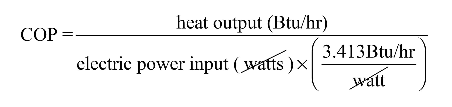
Formula 1
The slash marks across the units of (watts) indicate that they cancel each other out algebraically. That leaves the units of (Btu/h) in the top and bottom of the ratio. They also cancel each other out so that the results of the formula is a pure number (e.g., there are no units associated with COP). Because it’s a “unitless” value, the COP of a heat pump is the same regardless of what unit system is used (Imperial, Metric, …whatever).
It’s important to understand that the COP of a heat pump is an instantaneous value based on the heat pump’s instantaneous operating conditions. It changes whenever any of the heat pump’s operating conditions change. The only time a heat pump would have a constant COP is when the operating conditions are absolutely stable. In the case of an air-to-water heat pump, those conditions would be entering air temperature, air flow rate, entering water temperature, and water flow rate. Small changes in operating conditions yield small changes in COP, and vice versa. Over the course of a full heating season, there are wide changes in entering air temperature and entering water temperature. Changes in flow rates are possible, but typically less impactful in common applications. The bottom line: Don’t assume that a COP number listed in performance data, and based on some stated conditions, will hold constant, or vary by small amounts over a full heating season.
HSPF
The limited usefulness of an instantaneous COP value in predicting heating cost over time leads to other performance indices. One that’s commonly cited as a means of qualifying air-to-air heat pumps for incentive programs is Heating Seasonal Performance Factor (HSPF).
The HSPF of an air-to-air heat pump is determined by combining measured performance at different outdoor temperatures with rather complex calculations and assumptions about the size of the heat pump relative to design load, and the climate the heat pump operates in. Like AFUE, the assumptions built into the calculations, although consistent, do not necessarily apply when the heat pump is operating at conditions significantly different from those assumed. As such, its usefulness should be limited to making comparisons between different models of air-source heat pumps, rather than as an assured indicator of system operating cost. There are no HSPF ratings for water-to-water or air-to-water heat pumps since there is no “standard” that defines the hydronic distribution system operating conditions.
Seasonal Average COP
A more technically “grounded” metric for assessing the performance of a heat pump over a full heating season is called seasonal average COP. Although this term doesn’t have a recognized acronym, it does have a practical definition, given by formula 2.
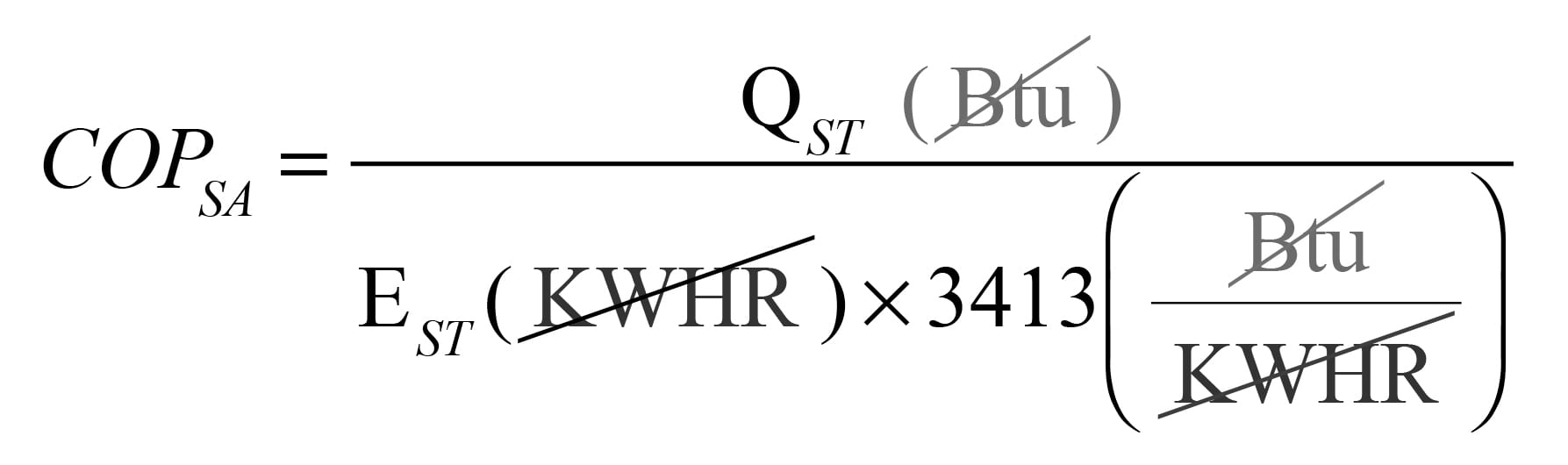
Formula 2
Where:
COPSA = seasonal average COP
QST= total heat delivered by heat pump over heating season (Btu)
EST = total electrical energy delivered to operate heat pump over heating season (KWHR)
Notice that the units of (KWHR) and (Btu) in Formula 2 both cancel out. This makes the seasonal COP a unitless number, as was the case for instantaneous COP.
Because it factors in many specifics rather than assumptions, the seasonal average COP is a better metric for estimating the operating cost of a specific heat pump, in a specific building, in a specific climate. Formula 3 shows how it would be used.
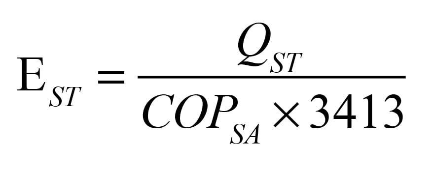
Formula 3
Where:
EST = total electrical input energy deliver to operate heat pump over heating season (KWHR)
QST= total heat delivered by heat pump over heating season (Btu)
COPSA = seasonal average COP of the heat pump
3413 = number of Btu per KWHR
There are two possible ways to get the seasonal average COP.
One is to accurately measure the total heat supplied from the heat pump over a full heating season, as well as the total electrical energy supplied to the heat pump over the same period, then used Formula 2. This is fine for an existing installation equipped with an accurate heat meter and electric energy meter.
However, most system designers and energy modelers who are trying to estimate operating cost need to know the seasonal average COP of a specific heat pump, supplying a specific building and heating system, in a specific climate, and they usually want to know this before committing to a specific product.
The only way to do this is by simulation. The typical approach uses bin temperature data for a specific location to “drive” equations that model the space heating load, as well as the heating capacity and COP of a specific heat pump. The total heating energy delivered by the heat pump would need to be estimated using building heating load models that include adjustments for the building’s internal heat gain from lights, equipment, cooling, sunlight, occupants, etc. Internal heat gain offsets part of the heat load and thus reduces the amount of heat required from the heat pump. The simulations may also include models for domestic water heating, cooling, and, in the case of air-source heat pumps, should include a derating factor for defrosting.
Figure 1 shows the results of such modeling conducted based on a nominal 4-ton low-ambient air-to-water heat pump supplying a building with a 36,000 Btu/h design load in three New York state climates.
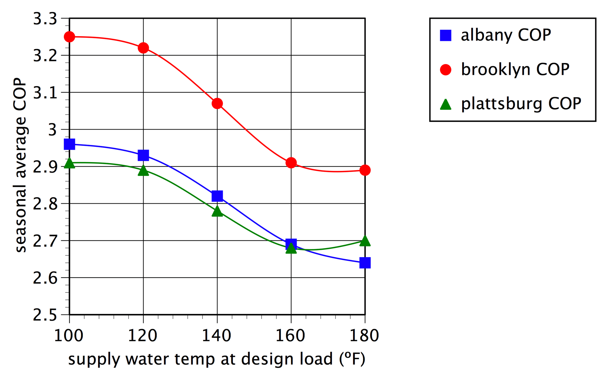
Figure 1
ENLARGE
The results show how lower water temperature distribution systems increase seasonal average COP, all other factors being equal. They also show the effect of climate. Plattsburg, New York, has an average of 8,044 °F•days with an outdoor design temperature of -8 °F, while Brooklyn has 4,880 °F•days and an outdoor design temperature of 15 °F.
The simulation model was based on outdoor reset control of the water temperature supplied by the air-to-water heat pump. The maximum allowed water temperature supplied by the heat pump was 130° F. Any space heating energy for distribution systems that, at times, required supply water temperatures above 130° F was assumed to come from electric resistance heating. The simulation also included corrections for defrosting, adjustments for internal heat gain in the building, and even factored in the wattage of the circulator creating flow between the heat pump and the remainder of the system.
Cooling Calcs
So far we’ve discussed performance metrics applicable to heating, but all modern heat pumps can also provide cooling. The performance metrics applicable to cooling include EER,Cooling COP and SEER:
A heat pump’s energy efficiency ratio (EER) is somewhat analogous to its COP. The main difference is that EER applies to cooling while COP applies to heating. The instantaneous EER of a heat pump is calculated based on Formula 4.
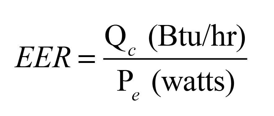
Formula 4
Where:
EER = energy efficiency ratio (Btu/hr/watt)
Qc =Total cooling capacity of heat pump (sum of latent and sensible cooling capacity) (Btu/hr)
Pe = electrical power input to heat pump (watts)
You’re probably looking at this formula and thinking that it looks very similar to the one for COP. You’re right. The difference is that EER has different units in the top and bottom of the ratio, whereas COP has the same units which ultimately cancel out. That’s just the way EER was originally defined. The higher the EER the greater the cooling output is, per watt of electrical energy input. Viewed another way, the higher the EER, the lower the electrical power input required for a given rate of cooling.
In Europe, the efficiency of a heat pump in cooling is simply called the cooling COP. I think this is more intuitive than EER because the concept of COP is being applied to both heating and cooling operation. You can get cooling COP by dividing EER by 3.413.
Like COP, EER is an instantaneous value that changes whenever the operating conditions of the heat pump change. It should not be used to estimate seasonal average performance. EER applies to air and water source heat pumps.
The seasonal average EER of an air-to-air heat pump is given by its SEER rating. The acronym SEER stands for Seasonal Energy efficiency Ratio. It’s calculated based on obtained the tested EER of an air-to-air heat pump at four different loading conditions, and then entering these tested values into Formula 5.

Formula 5
Where:
SEER = Seasonal Energy Efficiency Ratio (Btu/hr/watt)
EEE100 = tested EER of heat pump at 100% cooling load (Btu/h/watt)
EEE75 = tested EER of heat pump at 75% cooling load (Btu/h/watt)
EEE50 = tested EER of heat pump at 50% cooling load (Btu/h/watt)
EEE25 = tested EER of heat pump at 25% cooling load (Btu/h/watt)
The numbers (0.01, 0.42, 0.45, 0.12) are decimal percentages of the time, during the cooling season, that the heat pump is assumed to operate at the associated percentages of its full output. For example, 0.42 x (EER75) implies the heat pump runs for 42% of the cooling season at 75% of its rated capacity and the EER associated with that partial load condition. There’s no guarantee that these percentages of time apply to a given installation. However, they do define a consistent method for determining SEER, and thus allow consumers to make relative comparisons between competing air-to-air heat pumps.
Modern air-to-air heat pump with variable speed (“inverter”) compressors achieve higher EER valves under partial load conditions. This happens because less heat is dissipated across the condenser coil under partial load, and thus the refrigerant temperature in the condenser can be lower. Lower condenser temperatures improve the efficiency of any refrigeration process.
IPLV
Another performance index that’s similar in concept to SEER is called IPLV (Integrated Part Load Value). It’s defined in AHRI Standard 550/290 which applies to air-cooled chillers, primarily those used in larger commercial cooling applications. It uses the same coefficients and tested values of EER as the SEER ratings, but the conditions upon which those four EER values are established are based on specific outdoor air temperatures and leaving chilled water temperatures given with the AHRI 550/290 standard.
To date, there is no AHRI standard developed specifically for air-to-water heat pumps. However, some suppliers of air-to-water heat pumps with variable speed compressors publish IPLV values based on the AHRI 550/290 standard to demonstrate the inherent cooling efficiency gains associated with variable speed operation.
In my opinion, AHRI should be developing a new and specific standard that defines the heating and cooling performance metrics for air-to-water heat pumps. The North American market for these heat pumps is expanding with several new product offerings coming this year. The industry as a whole would benefit from a consistent standard that could be used by system designers as well as government agencies looking to establish baseline performance requirements that qualify air-to-water heat pumps for inclusion in incentive programs.
imantsu/iStock/Getty Images Plus via Getty Images.
John Siegenthaler, P.E., is a consulting engineer and principal of Appropriate Designs, in Holland Patent, New York. In partnership with HeatSpring, he has developed several online courses that provide in-depth design-level training in modern hydronic systems, air-to-water heat pumps and biomass boiler systems. The fourth edition of his textbook — “Modern Hydronic Heating & Cooling” — was released in April. For more information, visit www.hydronicpros.com.
